On Asymptotic Methods in Analysis: Prof. de Bruijn’s beautiful little book

For the past several days, I’ve been working my way through Prof. N.G. de Bruijn’s book Asymptotic Methods in Analysis; and I want to share some of the fun I’ve had reading it.

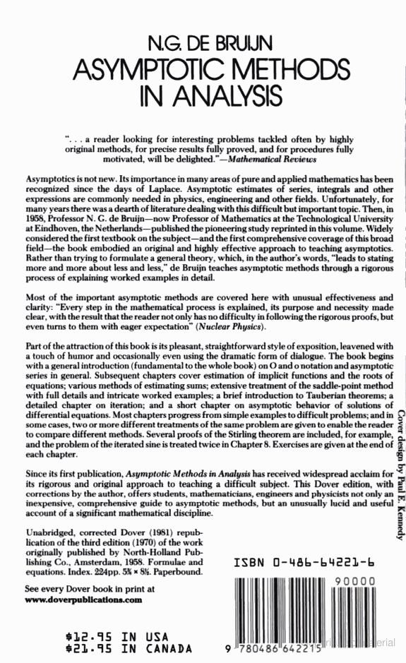
This post is not a review. The back cover has some reviews. Below are just fragments of what I’ve read so far and found fascinating. You could also consider this my attempt at trying to persuade you to get a copy of this beautiful little book! Dover does a great job at publishing inexpensive copies of these great works.

Prof. de Bruijn, his cycles, and average height of trees

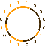
This book is by the same Prof. de Bruijn well-known, among other things, for his cycles , which are defined as following: An \(m\)-ary de Bruijn cycle/_ is a sequence of \(m^n\) radix-\(m\) digits such that every combinations of \(n\) digits occurs consecutively in the cycle. For example, one possible binary de Bruijn cycle of length \(2^4\) is: 0 0 0 1 1 1 1 0 1 0 1 1 0 0 1 0.

Treating this sequence as a cycle, notice that each of the 16 possible 4-bit patterns (0000 … 1111) appear exactly once in it. Knuth describes at least three interesting algorithms for generating such cycles in TAOCP Section 7.2.1.1 (now in print as TAOCP Volume 4A: Combinatorial Algorithms, Part 1.

There’s surely lots to say about Prof. de Bruijn’s work (including his cycles), but I’ll reserve them for future posts. Take a look, for example, at the index of TAOCP Vol I (perhaps also in other volumes) and you’ll see references to many of his results, sometimes framed as exercises. And if you enjoy asymptotic calculations and analyses of algorithms, you would find it interesting to read his co-authored paper (with Knuth and Rice) where it is shown that the average height of planted plane trees is:

\(\sqrt{\pi n} - {1\over2} + O(n^{-1/2})\).

This is also TAOCP Ex. 2.3.1–11, where the question is posed in terms of the average value of the maximum stack size consumed while running the usual in-order binary tree traversal, assuming all binary trees with n nodes are equally probable.

As an interesting note, Knuth in his musings on The Joy of Asymptotics (30 May 2000) said:

I’ve dedicated this book [Selected Papers on Analysis of Algorithms] to Prof. de Bruijn … in the Netherlands because he has been my guru … Ever since I got my PhD, I considered him my post-graduate doctoral advisor. Every time I had a problem that I got stuck on, I would write to him, and he would write me back a letter that would help me get unstuck. And that’s been going on for over fourty years now. So I dedicated this book to him. And what I want to talk to you about today is one of the things he has spent most of his life on – asymptotic methods.

Knuth's Selected Papers on Analysis of Algorithms

By the way, that paper deriving the cool formula for the height of trees is included in these Selected Papers (see Chapter 15).

The Book: A Pragmatic Exposition

I had got myself a copy of this book several years ago after first reading about it in the section on asymptotic calculations in TAOCP (Sec 1.2.11.3). But unfortunately, the book suffered the same fate as countless others – it just kept resting on my bookshelf. But a few days ago, I decided to give it a try.

A brief history. As described in its preface, this book grew out of lectures given in 1954–55 and was first published in 1958. The Dover edition I have is a reprint of the third edition from 1970.

Most computer programmers are familiar with the Big-O notation, or the Bachmann-Landau notation, for analyzing space/time-complexity of an algorithm. Among other things, this book talks of the tricks involved in getting precise asymptotic bounds once we have reduced the problem at hand to, say, a sum or an integral.

This is a pragmatic book – its focus is on demonstrating general techniques by working out several examples in detail (sometimes in more than one way) rather than expounding highly generalized theories of analysis. In this context, I found these lines from the preface reassuring:

Usually in mathematics one has to choose between saying more and more about less and less on the one hand, and saying less and less about more and more on the other. In a practical subject like this, however, the proper attitude should be to say as much as possible in a given situation.

From my reading, at certain places it, of necessity, assumes a basic knowledge of analysis and complex variable theory. Other than that, it is a fairly elementary treatment. Tangent: Feynman made a great point in one of his lectures

“Elementary” means that very little is required to know ahead of time in order to understand it, except to have an infinite amount of intelligence.”

It’s a small book (200 pages) with very few exercises and so can be read in about two weeks, if you read an hour a day. And since there are lots of cliff-hanging moments (well, to the extent a book on analysis can have!) and the reader is left wondering how a tricky sum/integral would be tamed, your might be compelled to finish it even sooner!

de Bruijn has a good sense of humor too. At the start of the first chapter, when trying to answer the question “What is Asymptotics?”, he says:

The safest and not the vaguest definition is the following one: Asymptotics is that part of analysis which considers problems of the type dealt with in this book.

Didn’t see that one coming!

And while the book is tiny, it covers lots of tricks & techniques. So, to give my interested readers a taste, I’ve picked a couple of my favorite from the first chapter. All examples are de Bruijn’s.

Uniform Estimates

Uniformity of estimates is this little thing that keeps popping up every so often when analyzing the asymptotics of some characteristic of an algorithm. But it is rarely explained what it means or why uniformity is crucial to the application at hand. Grown ups are supposed to know what uniformity is, I suppose.

Before looking at uniformity, let’s recap the definition of the \(O\)-notation. We say:

\[f(x)=O(\phi(x))\qquad(x\rightarrow\infty)\]

to mean the existence of numbers \(a\) and \(A\) such that:

\[\left\lvert f(x)\right\rvert \leq A \left\lvert\phi(x)\right\rvert\qquad \text{whenever}\quad x > a\]

The thing to note in this definition is that the \(O\)-notation implies two implicit constants, \(A\) and \(a\).

Returning to the question of uniformity, suppose \(k\) is a positive integer and \(f(x)\) and \(g(x)\) are arbitrary functions. Then:

\[( f(x) + g(x) )^k = O( ( f(x) )^k + ( g(x) )^k)\]

because \(\left\lvert(f+g)^k\right\rvert\leq (\left\lvert f\right\rvert+\left\lvert g\right\rvert)^k\leq (2\max(\left\lvert f\right\rvert, \left\lvert g\right\rvert))^k\leq 2^k(\left\lvert f\right\rvert^k + \left\lvert g\right\rvert^k)\).

Rewriting the last line as: \((f(x) + g(x))^k\leq A\left\lvert f(x)\right\rvert ^k + B\left\lvert g(x)\right\rvert^k\), we see that the implicit “constants” \(A\) and \(B\) depend on the parameter \(k\). We call such an estimate non-uniform.

On the other hand, in the asymptotic relation (with \(k\) again being a positive integer):

\[({k\over{x^2+k^2}})^k=O({1\over{x^k}})\qquad (x > 1)\]

the implicit constant in the \(O\)-notation is independent of k, since we have \(({k\over{x^2+k^2}})^k\leq ({k\over{2kx}})^k\leq {1\over{x^k}}\).

Hence if we write \(({k\over{x^2+k^2}})^k\leq {A\over{x^k}}\), with \(x > 1\), we can choose \(A\) to be 1. In such a case – when the hidden constants in the \(O\)-notation do not depend on the parameter \(k\) – the estimate is called uniform. This requirement is much like that of uniform convergence or uniform continuity in analysis.

So why trouble oneself with uniformity? Here’s one case where uniform estimates prove helpful: In “balancing” the asymptotic terms of a sum evenly to achieve a tight bound.

For instance, if we have somehow shown that \(f(x) = O(x^2t) + O(x^4t^{-2})\) with \(x, t > 1\) and where \(t\) is a parameter. If the formula holds uniformly, we can get a tight bound by reasoning as follows: When \(t\) is small, the first part, \(O(x^2t)\), is small, but the second part, \(O(x^4t^{-2})\), is large; the reverse holds if \(t\) is large. Hence we wish to find a “balance” that minimizes the sum of the \(O(\cdot)\) terms. And this happens when both the terms are asymptotically equivalent. So to achieve such a balance, we simply equate the two expressions \(x^2t = x^4t^{-2}\), giving \(t=x^{2/3}\), and we finally get \(f(x) = O(x^{8/3})\). Notice that because of uniformity, the four hidden constants (\(A_1\), \(a_1\), \(A_2\), \(a_2\)) of the two \(O(\cdot)\) do not vary when we vary the parameter \(t\). If the two original \(O(\cdot)\) estimates had not been uniform; that is, had their hidden constants (implied by the \(O\)-notation) varied with \(t\), we wouldn’t have been able to apply this simplistic “balancing” idea. For instance, while for small \(t\), the \(x^2t\) term might have been small, the hidden constant \(A_1\) in \(O(x^2t)\) might have grown, leading to unpredictable overall behavior. The good thing about uniform estimates is that they are sometimes more useful; but proving uniformity might require a more careful analysis.

Asymptotic Series and Convergence: Some Curious Facts

An asymptotic series or asymptotic expansion for a function \(f(x)\) is a formula like:

\[f(x) \approx c_0\phi_0(x) + c_1\phi_1(x) + c_2\phi_2(x) + \ldots \qquad (x\rightarrow\infty)\]

where, as \(x\rightarrow\infty\),

\[\phi_{j+1}(x)=o(\phi_j(x))\qquad j\geq 0\]

and

\[f(x) = c_0\phi_0(x) + c_1\phi_1(x) + \cdots + c_{n-1}\phi_{n-1}(x) + O(\phi_n(x))\qquad (n\geq 0)\]

That is, the asymptotic expansion for \(f(x)\) is a series of functions such that if we truncate the series at the \(n\)th term, the partial series provides an approximation to \(f(x)\) (as \(x\rightarrow\infty\)) with the error term asymptotically bound by the first truncated function. The Euler-Maclaurin formula is one way to get such an expansion. de Bruijn mentions other techniques in the book.

A large class of examples of asymptotic expansions are convergent power series, like:

\[\exp(z) = 1 + z + {z^2\over2!} + {z^3\over3!} + \cdots\qquad (\left\lvert z\right\rvert\rightarrow0)\]

But there could be asymptotic expansions that are not convergent power series. And with such asymptotic expansions, some curious things can happen:

The series of the asymptotic expansion need not be convergent.
If the series does converge, its sum need not be equal to \(f(x)\)
It is even possible to have \(f(x)\) and \(\phi_j(x)\)’s such that the sum of the series does not have the series as its own asymptotic expansion!

The essential reason for these seemingly strange facts, as de Bruijn explains, is:

… that convergence means something for some fixed \(x_0\) whereas the \(O\)-formulas are not concerned with \(x=x_0\), but with \(x\rightarrow\infty\). Convergence of the series, for all \(x > 0\), say, means that for every individual \(x\) there is a statement about the case \(n\rightarrow\infty\). On the other hand, the statement that the series is the asymptotic expansion of \(f(x)\) means that for every individual \(n\) there is a statement about the case \(x\rightarrow\infty\). For example, when \(f(x) = \int_1^x{e^t\over t}dt\) the asymptotic expansion of \(e^{-x}f(x)\) is \({1\over x} + {1!\over x^2}+ {2!\over x^3} + {3!\over x^4} + \ldots \quad (x\rightarrow\infty)\) but the series converges for no value of \(x\).

Conclusion

The book covers lots of useful stuff. In particular, It talks about Lagrange’s inversion formula (using which we can solve for the tree function), it has a especially thorough treatment of the saddle-point method. And much much more.