Fun with ZDDs: Notes from Knuth’s 14th Annual Christmas Tree Lecture

In this entry, I’ll record the important ideas Knuth presented in his 14th Annual Christmas Tree Lecture, part of his regular Computer Musings.

Like all other “musings”, this one included some fascinating anecdotal bits (no pun intended) and Knuth’s good sense of humor was sprinkled throughout; but most noticeable was his infectious enthusiasm for the topics he spoke about. The preface to Volume 4 (printed in Fascicle 0) begins with:

The title of Volume 4 is Combinatorial Algorithms, and when I proposed it, I was strongly inclined to add a subtitle: The Kind of Programming I Like Best.

His excitement for these topics clearly showed in the lecture. It is a must-watch for anyone interested in The Art of Computer Programming (especially Volume 4 on Combinatorial Algorithms), or interested in learning a very useful data structure for combinatorial applications — ZDDs.

ZDDs

ZDDs (Zero-suppressed Binary Decision Diagrams) were introduced by Shin-Ichi Minato in 1993, about seven years after Randal Bryant introduced his key ideas of the BDD data structure; one of which was that keeping the BDD both reduced and ordered is important in practice. In his “Fun with BDDs” musing (this June), Knuth mentioned that this 1986 paper of Bryant’s took computer science almost by storm; remaining the most-cited paper in the field for many years.

Minato’s idea (of zero-suppression in BDDs) was motivated by his observation that when working with combinatorial objects, very often tests in BDDs have to be made just to ensure a potentially large number of variables are FALSE. So, in ZDDs, we just “skip over” any node whose HI pointer leads to \(\bot\) (the FALSE sink) — if having \(x_j\) TRUE results in the subfunction rooted at \(x_j\) to become FALSE, then we skip testing \(x_j\) altogether. That’s the basic difference between BDDs and ZDDs. And while ZDD theory is much like the BDD theory, it differs sufficiently in the sense of requiring a different “mind-set”.

The pre-fascicle 1B that discusses BDDs and ZDDs is available from Knuth’s website (direct link). That pre-fascicle is a 140-odd page booklet with more than 260 exciting exercises! It will be published as part of fascicle 1 (Knuth said it’ll go to printing around the end of January 2009); fascicle 1 would in turn form part of Volume 4A (along with the already published fascicles 0, 2, 3 and 4).

Update: TAOCP Volume 4A: Combinatorial Algorithms, Part 1 is now in print. In addition to the material on BDD and ZDD techniques (described in this post), it includes a subsection on bitwise tricks and techniques, including broadword computing (formerly known as “Platologic computing”). In Knuth’s own words, it is “cram-packed with lots of new stuff among nearly 500 exercises and answers to exercises.”

Families of subsets and their ZDD representation

BDD is a data structure for (representing, manipulating, working with) boolean functions. ZDD, on the other hand, is a data-structure for what Knuth calls Families of Sets – a large number of combinatorial problems are based on studying families of sets (which are just Hypergraphs). Families of sets are another way of looking at boolean functions since there’s a natural one-to-one correspondence between the two — the solutions of a boolean function (the set of n-tuples of boolean values \(x=(x_1,\ldots,x_n)\) such that \(f(x)\) is TRUE) correspond to family of subsets, with each solution corresponding to a subset where \(j\) belong to the subset iff \(x_j=1\) (see TAOCP Exercise 7.1.4 — 203(b)).

But even though the families of sets can be encoded as boolean functions, it is sometimes better to think of them directly as families of sets, rather than in boolean sense. This is the thinking cap we’ll put on when working with ZDDs. Families of subsets are taken from a well-ordered universe \(U\). We use the following rules to represent those using ZDDs (again, see TAOCP Exercise 7.1.4 — 203):

The Empty Family, \(\phi\), is represented by \(\bot\) (the FALSE sink node).
The Unit Family (the set comprising just the empty set), \(\{\phi\} = \epsilon\), is represented by \(\top\) (the TRUE sink node).
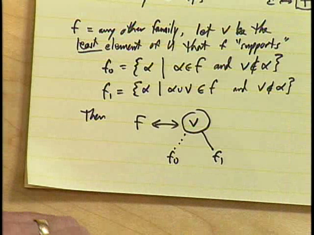
If \(f\) is any other family (besides empty and unit), we know that it is nonempty, and that at least one of its members is in turn nonempty. In that case, let \(v\) be the least element of universe \(U\) that \(f\) supports — that \(v\) appears in at least one set in \(f\) (see answer to TAOCP Exercise 7.1.4 — 197 for the definition of supports). Then define sub-families \(f_0\) and \(f_1\) of \(f\) with \(f_0=\{\alpha \mid \alpha\in f\ \wedge\ v\notin\alpha\}\) and \(f_1=\{\alpha \mid \alpha\cup\{v\}\in f\ \wedge\ v\notin\alpha\}\). These sub-families correspond to those sets that don’t and do contain \(v\). Then, inside the computer, the family \(f\) corresponds to a zead (ZDD-node) labeled \(v\) with LO and HI branches going to the ZDD representations of \(f_0\) and \(f_1\) respectively. Notice the recursive definition (see Knuth’s diagram).

Throughout the talk, Knuth took up various problems, and worked them out in real-time for everyone to follow, rather than putting up a bunch of slides with everything already worked out. This is one of the beauties of his musing lectures — it’s interactive. While Knuth works his way through the problems, the audience can work with him or with their own pencil and paper. And it’s even more convenient when watching the recorded session over net, where one can pause, work the problem out, and then play to see if they got it right, and go back etc.). Knuth also joked about how he sometimes had to sit through presentations where the speaker doing PowerPoint would whiz through the slides a bit too fast. So, anyway, the most instructive (and most enjoyable) way to understand these examples, I think, would be to just watch the video and work them out yourself (possibly after going through the relevant material in the pre-fascicle).

Example 1. ZDD of a function

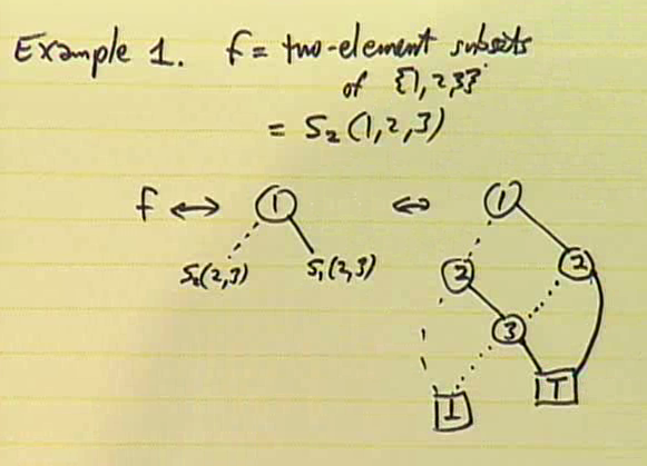
Here, Knuth took the example of family \(f\) = the family of 2-element subsets of \(\{1,2,3\}\), that is, \(f=S_2(x_1,x_2,x_3)\) and explained how to construct its ZDD (see diagram above). The family \(f\) is \(\{\{1,2\},\{1,3\},\{2,3\}\}\), so its least support is \(1\). The \(f_0\) and \(f_1\) families turn out to be \(S_2(2,3)=\{\{2,3\}\}\) and \(S_1(2,3)=\{\{2\},\{3\}\}\) respectively. So we have LO and HI branches (dotted and solid lines in the diagram above) going from \(1\) to the ZDD of \(f_0\) and \(f_1\) that we recursively construct. Notice that no node with the same (V, LO, HI) triple appears twice in our data structure (that is, the diagram is reduced). So although Knuth is giving a Christmas “Tree” lecture, a ZDD is not a true tree because overlapping subtrees are combined into one — rather, a ZDD is a DAG (directed acyclec graph).

Example 2. ZDD-base and its computer representation

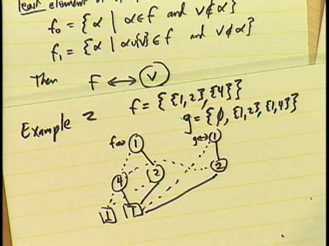
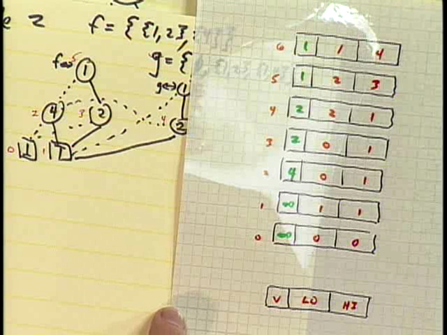
Ex. 2: Representation of ZDD-base (@31m30s)

When working on real problems, there’re usually many functions we’re working with simultaneously. So instead of a ZDD representing a single function, we really have a ZDD-base where common zeads are shared across functions. Knuth constructed the ZDD-base of the two functions \(f=\{\{1,2\},\{4\}\}\) and \(g=\{\phi,\{1,2\},\{1,4\}\}\). Inside a computer, a ZDD is represented as a linked structure, where each node of the ZDD, zead, is represented as a record with 3 fields: V (Variable ID#), LO (Low Pointer), HI (High Pointer). Sink nodes have their V field set to \(\infty\), with LO and HI fields pointing back to them (see diagrams above).

ZDD-bases satisfy certain laws:

No two nodes have the same triple (V, LO, HI) — that is, the structure is reduced.
No node has HI = 0, except sink \(\bot\) — this is the reason Minato called it zero-suppressed — the idea is to “skip over” such nodes
For non-sinks f, V(LO(f)) > V(f) and V(HI(f)) > V(f) when f > 1 — that is, the nodes are ordered with V-fields are always increasing as we walk down the structure

ZDD-bases, which though conceptually easy to understand, are non-trivial to implement efficiently because behind the scenes, lots of things have to be taken care of:

New nodes are born and old ones die — nodes have to be efficiently allocated, ref-counted and garbage-collected.
The UNIQUE-table (hash-table for (V, LO, HI) triple) has to be efficiently maintained and kept fresh with any changes made to the ZDD. A memo-cache has to be similarly maintained for caching recently computed results (like AND/OR of function).

Knuth’s BDD15 (literate) program, available from his Downloadable Programs page should provide an instructive study of the issues and techniques involved. I gained a lot of clarity on tricky BDD topics like ref-counting nodes, reordering of variables, efficient function composition etc, by studying Knuth’s BDD14 program. I used it as a reference whenever I got stuck anywhere with my own BDD implementation. BDD15 should be equally useful, and I plan to find time to study it soon.

Example 3. Nested parentheses

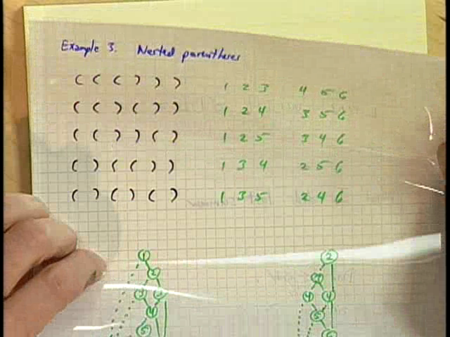
Nested parentheses are a natural way to describe tree structures (LISP being a good example). In this example, Knuth showed how to represent the 5 ways to correctly nest 3 sets of parentheses using a ZDD:

Parenthesis Nesting	ZDD subset
`( ( ( ) ) )`	\(L_1L_2L_3R_4R_5R_6\)
`( ( ) ( ) )`	\(L_1L_2R_3L_4R_5R_6\)
`( ( ) ) ( )`	\(L_1L_2R_3R_4L_5R_6\)
`( ) ( ( ) )`	\(L_1R_2L_3L_3R_4R_4\)
`( ) ( ) ( )`	\(L_1R_2L_3R_4L_5R_6\)

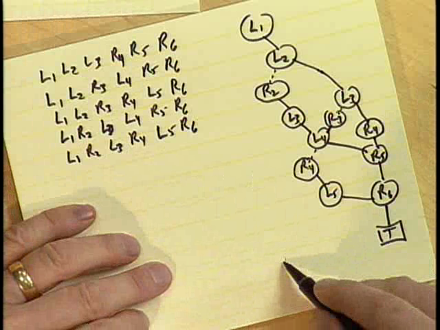
In this representation, subscripts correspond to positions in the string with \(L\)/\(R\) denoting the kind of parenthesis. The ZDD for this represents a family of 5 sets (each containing 6 elements). In the ZDD, the variable ordering used is \(L_1,R_1,L_2,R_2,\ldots,L_6,R_6\) (see the diagram above).

For \(n=3\) parentheses pairs, the ZDD contains 14 nodes and don’t appear to save a whole lot. However, if we consider \(n=24\) parentheses pairs, the ZDD of 602 nodes represents 1.3 trillion solutions! This compact ZDD structure encodes all those solutions without having to store them explicitly; and yet we can ask questions about the solutions. Like, say, analyze solutions that contain \(L_3\). The figure 1.3 trillion comes because the number of ways to nest \(n\) pairs of parentheses in a balanced way is the Catalan number, \({1\over{n+1}}\binom{2n}{n}\). See TAOCP Exercises 2.2.1 — 2, where a proof of this fact is given using a “reflection principle”; and also Eq. 2.3.4.4 — (14), which deals with enumeration of binary tree.

So, using only a small space, ZDDs can represent large families of combinatorial sets of interest, allowing efficient operations on these families and helping solve problems related to them. For example, if a family of sets is represented as a ZDD, one can quickly (in terms of the size of the ZDD) find a random set of the family.

Operations on families and Family Algebra

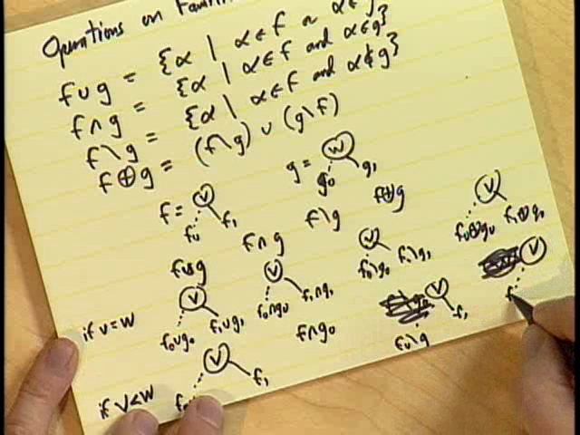
(This is actually Ex. 7.1.4 — 203, 204.) People from different branches of combinatorics have different operations they want to perform on families of sets. The usual ones are:

Union: \(f\cup g=\{\alpha\mid\alpha\in f\ \vee\ \alpha\in g\}\)
Intersect: \(f\cap g=\{\alpha\mid\alpha\in f\ \wedge\ \alpha\in g\}\)
Difference: \(f\setminus g=\{\alpha\mid\alpha\in f\ \wedge\ \alpha\notin g\}\)
Symmetric Difference: \(f\oplus g=(f\setminus g)\cup(g\setminus f)\)

All four operations can be efficiently implemented given the ZDDs of \(f\) and \(g\) using an easy recursive process based on the smallest support for the two functions. The implementation can be sped up using a memo-cache.

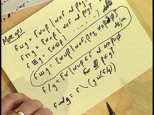
In addition to the ones above, more operations are possible: \(f\sqcup g\) (meet), \(f\sqcap g\) (join), \(f\boxplus g\) (delta), \(f/g\) (quotient), \(f\mod g\) (remainder). Knuth said he had recently discovered another binary operation that he thinks might prove useful. He likes to call it disjoin since it is similar to the join operation, but works on disjoint sets:

\[f\star g=\{\alpha\cup\beta \mid \alpha\in f, \beta\in g, \alpha\cap\beta=\phi\}\]

The \(\star\) is not what Knuth uses as the symbol for disjoin (for the correct symbol, see his hand-written version in the snapshot above), but I haven’t yet figured out the \(\TeX\) name for that symbol.

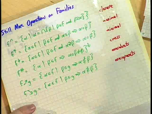
Even more operations on families are possible (see Exercise 7.1.4 — 236): \(f^{\cap}\) (closure), \(f^{\uparrow}\) (maximal elements), \(f^{\downarrow}\) (minimal elements), \(f\nearrow g\) (nonsubsets), \(f\searrow g\) (nonsupersets), \(f^{\#}\) (cross elements). Seeing all these funny symbols, somebody chimed in an obligatory APL joke; somebody else mentioned “family values” in connection with family algebra. People were certainly having fun!

Towards the end, Knuth mentioned various applications of the ideas he had spoken of earlier.

Application 1. Exact Cover Problems

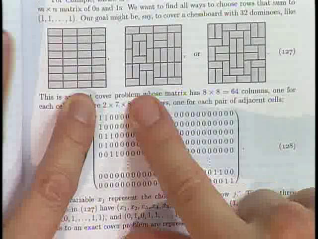
Appl. 1: Covering a chessboard (@54m30s)

Exact Cover Problems essentially involves selecting rows from a given boolean matrix in such a way that each column among the selected rows has exactly one 1. A popular example of this kind of problem is Sudoku. Knuth, in an earlier musing, mentioned an efficient dancing links algorithm for solving such problems.

In the present musing, Knuth showed the examples of covering an 8x8-chessboard with 32 dominoes [7.1.4 — displays (127) to (129)]; covering with monominoes/dominoes/trominoes [display 7.1.4 — 130]; or covering with dominoes of three colors (red, white, blue) with no adjacent dominoes of the same color [Exercise 7.1.4 — 216].

Application 2. Dictionaries

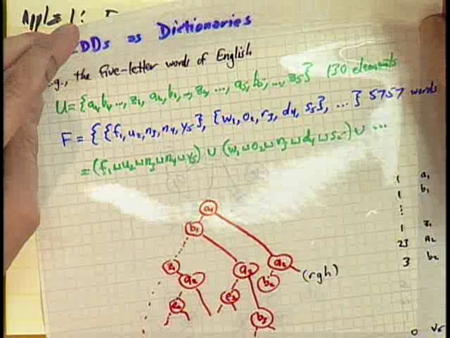
Appl. 2: ZDDs as Dictionaries (@1h03m15s)

Appl. 2: Query ZDD words dict (@1h15m30s)

Knuth showed how, with 5*26 = 130 variables, it is possible to store all five-letter words of the SGB (Stanford GraphBase) in a ZDD, and perform operations such as:

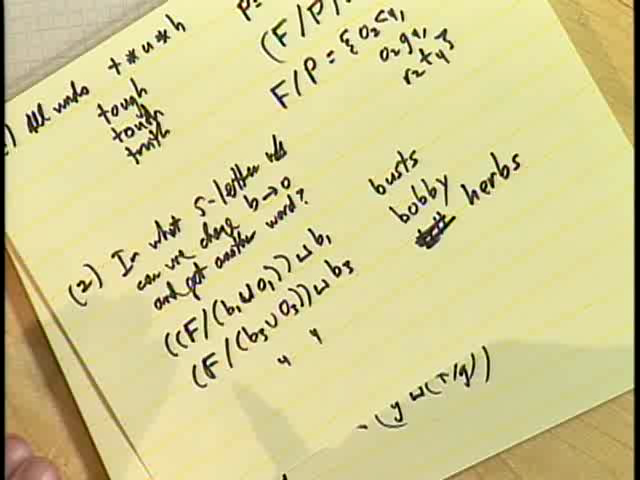
Querying for words that match the pattern t?u?h. This involves using family algebra on ZDDs to compute \((F/P)\sqcup P\) where \(P\) is the “pattern” \(t_1\sqcup u_3\sqcup h_5\).
Finding all words such that when the letter b in it is changed to the letter o, we still get a valid five-letter word. This involves computing \((F/(b_j\cup o_j))\sqcup b_j\), which gives words like busts (\(j=0\)), herbs (\(j=3\)) etc.

Application 3. Graph problems

Knuth illustrated application of ZDDs to graph problems by showing how it can be used to find various constrained arrangement of queens on a chessboard (queens-graph): kernels, maximal cliques, dominating sets etc. [See Exercise 7.1.4 — 241]. All these operations can be implemented using ZDDs and family algebra operations (see Knuth’s sheet). Letting \(g\) to be the family of edges of a graph/hypergraph (such that members of \(g\) are subsets of the sets of vertices \(V\)):

Independent Sets are \(f=\wp\searrow g\) (Knuth uses Weierstrass P \(\wp\) to denote the power set \(2^V\))
Maximal Independent Sets (or Kernels) are the maximal elements \(f^{\uparrow}\) of the independent sets
Dominating Sets are \(d=\{\alpha\mid\alpha\cap\Gamma(x)\neq\phi\ \forall x\in V\}\) where \(\Gamma(x)=\{\alpha\in g\mid x\in\alpha\}\)
Minimal Dominating Set is \(d^{\downarrow}\)
Maximal Induced Bipartite Subgraphs is \((f\sqcup f)^{\uparrow}\)

Knuth had so much interesting stuff to talk about. But he had spoken for 90 minutes already — so he decided to stop.

I’ve been studying fasc1b for about three months now and have been enjoying myself thoroughly — learning new data-structures & proof techniques, developing my own BDD-base, working out the programming exercises, playing with Conway’s game of Life, coloring graphs and more. I’m still only two-thirds through with the exercises (that total to a respectable 263) — just about to start working on the ZDD exercises. I hope to be able to work my way through the exercises by the end of this year.